
Section analysis
Run ultimate and serviceability limit state checks, prestress analysis, fire design, and moment-curvature analysis on concrete sections.
Overview
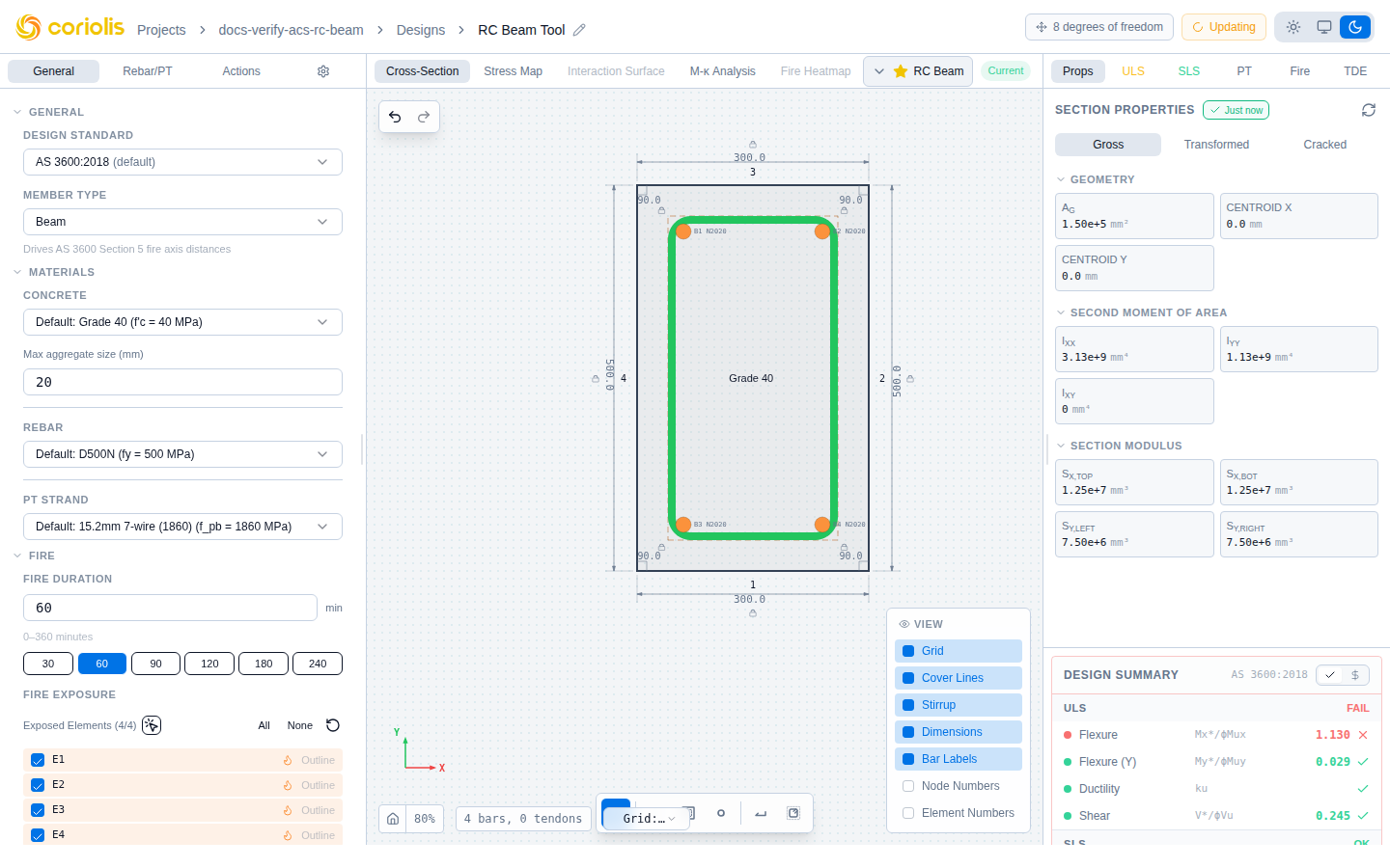
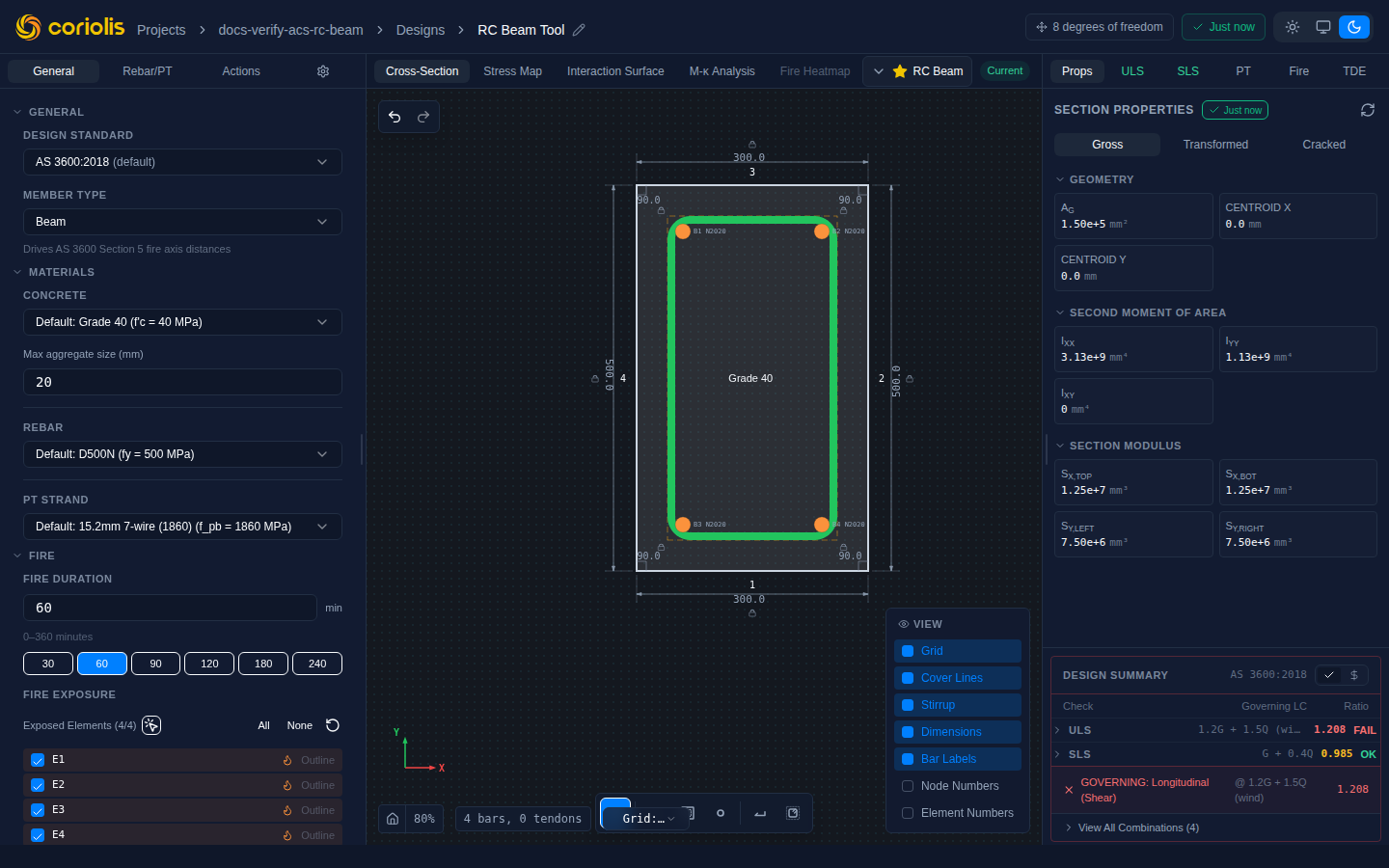
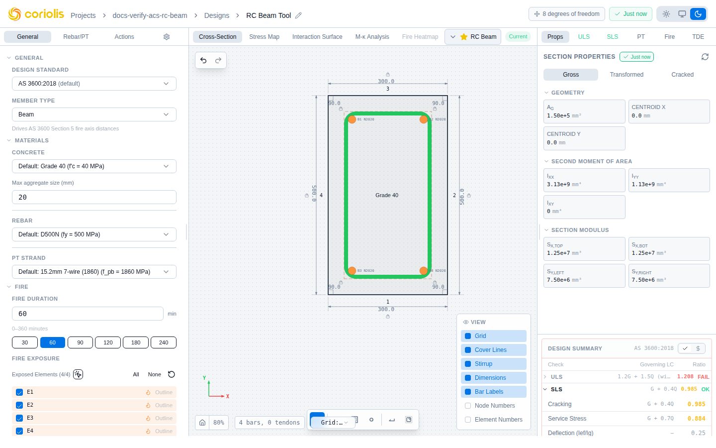
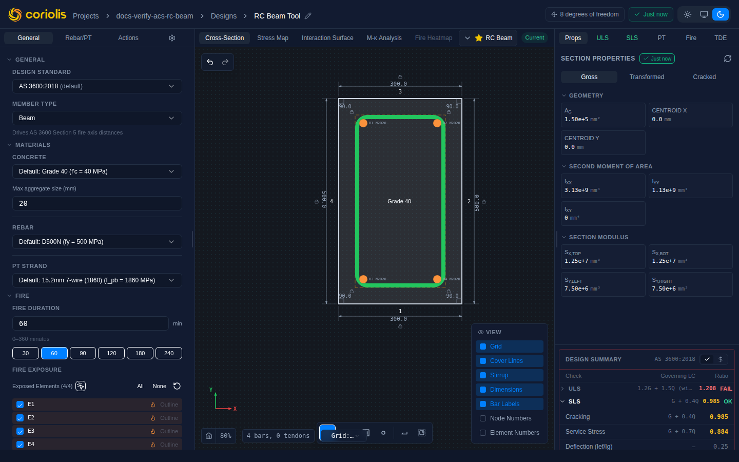
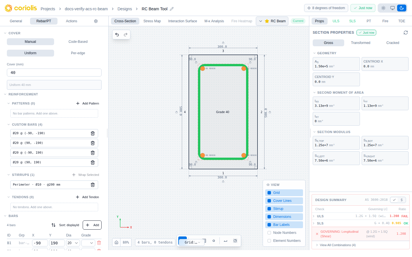
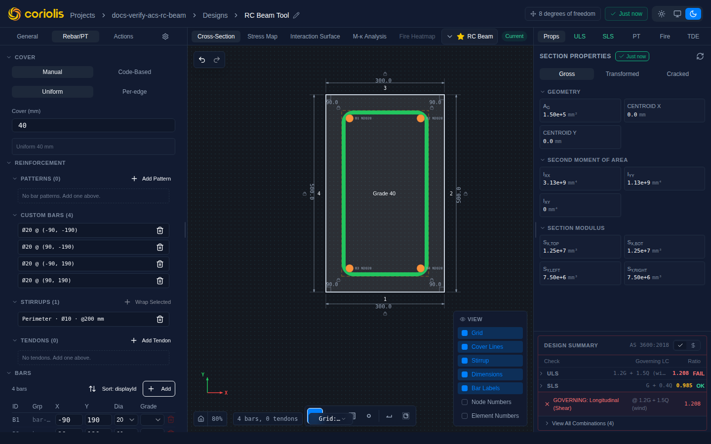
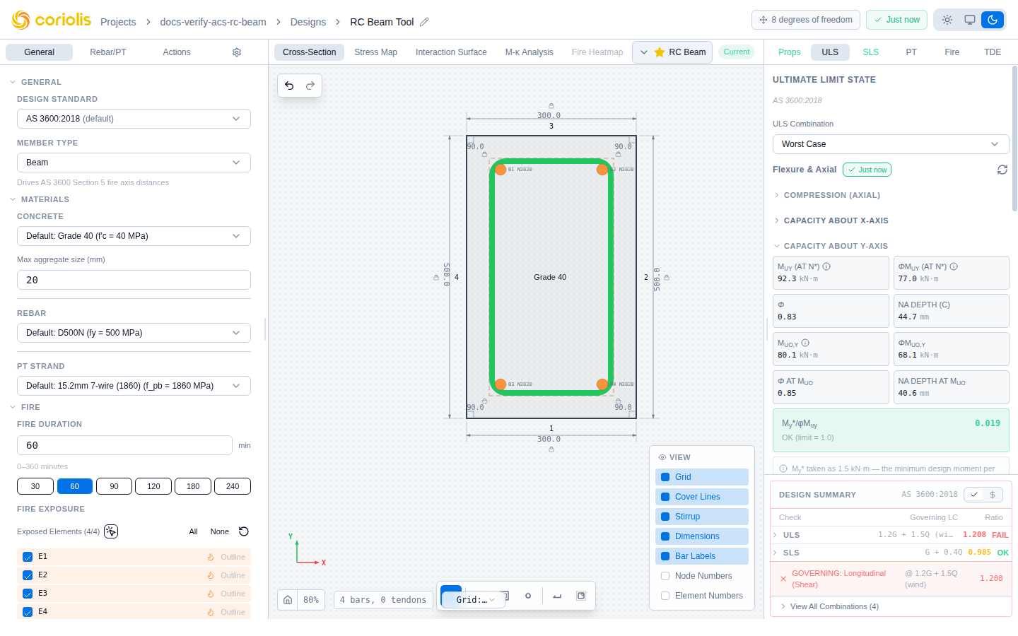
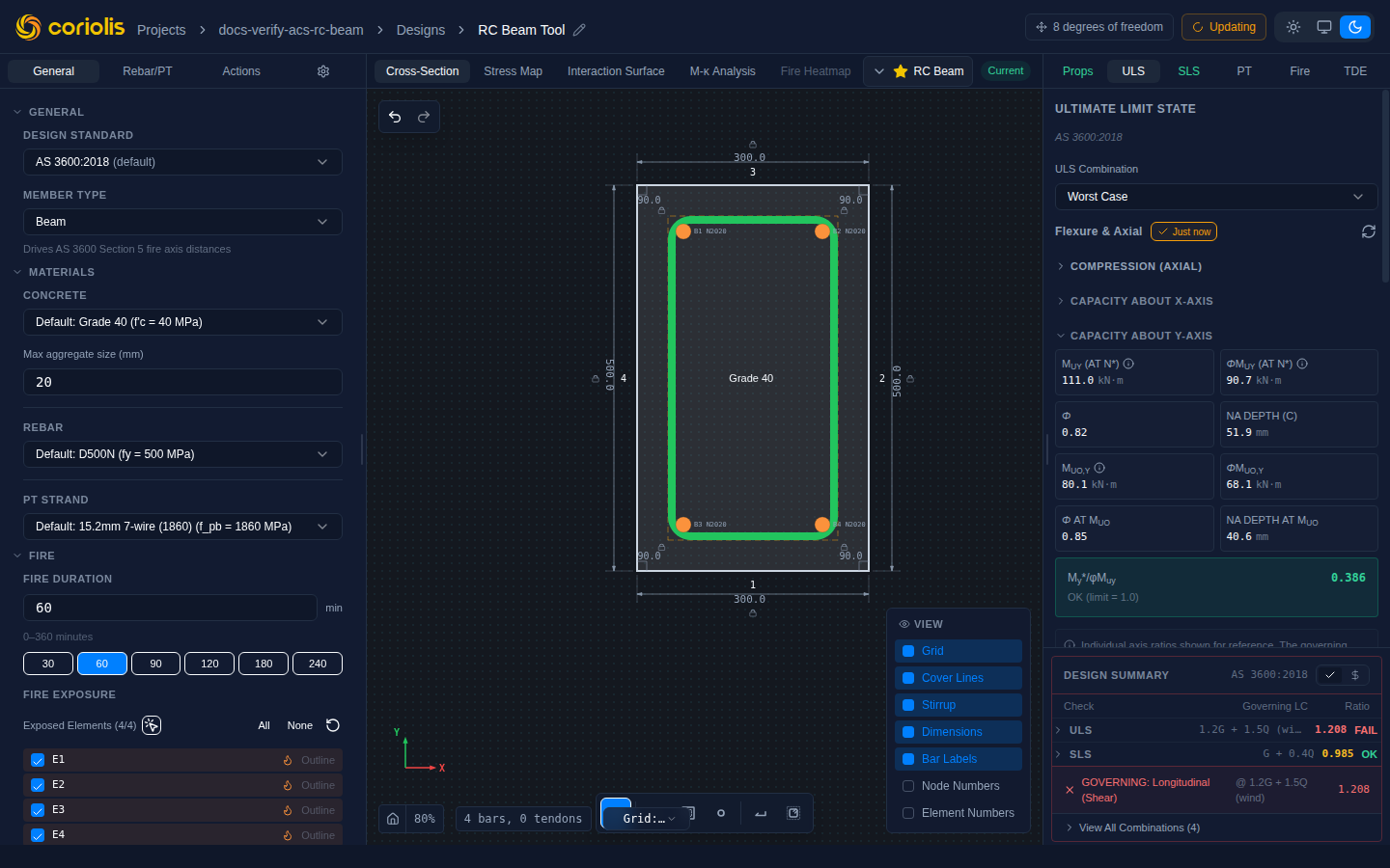
Once you have defined the section geometry, reinforcement, and materials, ACS runs design checks automatically as you enter or modify design actions. Results appear in the right panel, organised by limit state.
All calculations re-run with a short debounce delay after any input changes. You can also force a full refresh with Ctrl+Shift+Enter.
ACS calculations are reconciled to AS 3600:2018 Amendment 2:2021 for Australian projects. See Design standards for a full code-by-code comparison.
Applied loads
Open the Applied Loads panel to define design actions. Select the member type to control which load fields are visible:
| Member type | Visible loads |
|---|---|
| Beam | , , |
| Column | , , |
| Beam-Column | , , , , , |
Sign conventions
ACS follows the platform-wide canonical:
- Positive = compression (the section is being pushed together).
- Positive = sagging about the -axis = compression at the top face (). Tension at the bottom face.
- Positive = bending about the -axis with compression at the left face (). Tension at the right face.
- Combined positive → peak compressive stress lands in the top-left quadrant.
- Concrete and steel stresses reported by ACS use σ > 0 = compression (the concrete-design convention).
- Neutral axis depth (or ) is always measured from the compression face — for positive that is the top face downward.
Hover the Mx or My label in the Applied Loads panel to see the per-field tooltip, or look at the Y↑ X→ axis indicator in the bottom-left of the canvas.
For the full canonical (strain field, curvature signs, transcribing from external sources) see Platform — Sign and axis conventions.
Load combinations
ACS supports multiple load combinations, each tagged with a limit state:
| Limit state | Purpose | Example |
|---|---|---|
| ULS | Ultimate strength checks (flexure, shear, interaction) | 1.2G + 1.5Q |
| SLS | Serviceability checks (stress, crack width, deflection) | G + 0.7Q |
| Fire | Fire-rated capacity checks at elevated temperature | G + 0.4Q (fire) |
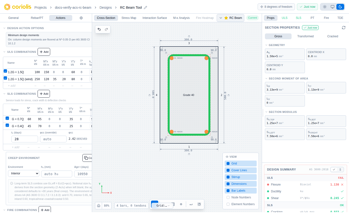
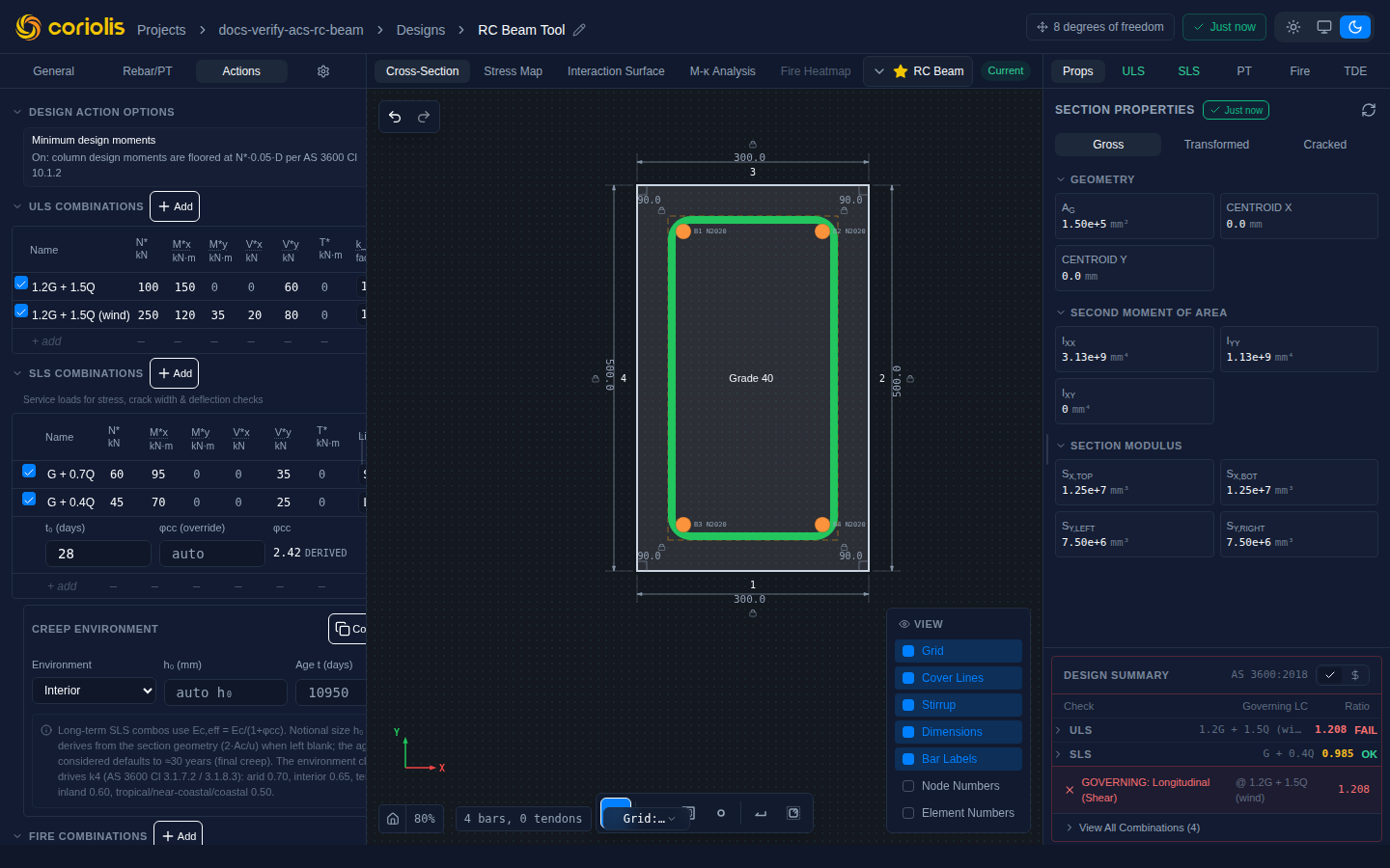
Type directly into the ghost row at the bottom of each limit-state table to add a new combination. Entering a value in any ghost-row cell immediately materialises a real row, seeded with that value, and keeps focus in the same cell so you can continue editing without interruption.
Within a row, Tab moves to the next cell (wrapping to the next row at the end), Shift+Tab moves back, and Enter commits the current cell and advances focus downward. The ghost row at the bottom is always available — pressing Tab through the last real row lands on it.
Each combination also has an active/inactive toggle — inactive combinations are skipped when ACS selects the governing check.
The governing combination for each check type is identified automatically in the Design Summary.
k_φ — capacity reduction modifier (AS 3600 Amendment 2:2021)
When the AS 3600 design code is selected, each ULS load combination has a compact k_φ inline dropdown in the trailing column of the load table:
| k_φ value | Factor | When to use |
|---|---|---|
| Full | 1.0 | The column is short (Cl. 10.3) and |
| Reduced | 12/13 ≈ 0.923 | All other cases (default) |
The k_φ class modifies the compression-controlled capacity reduction factor: .
This input gives you direct control over the Amendment 2:2021 capacity class per load combination, independently for each combination. For short columns under predominantly live load (), use Full; for long columns or gravity-dominated loads, use Reduced.
SLS sub-state — limit-state type per combination (AS 3600)
Each SLS load combination carries a sub-state inline dropdown in the trailing column of the SLS table. The sub-state controls whether long-term time-dependent behaviour is activated for that combination:
| Sub-state | Behaviour |
|---|---|
| SLS | Short-term checks. Creep and shrinkage terms are not applied. |
| QP (quasi-permanent) | Long-term checks. Triggers and terms in crack-width and deflection calculations. |
Selecting QP expands a second row beneath the combination for time-dependent inputs: the concrete age at loading , an optional override, and the derived final design creep factor. Short-term (SLS) rows collapse to a single line.
The ACI 318 and EN 1992 equivalents are LT (long-term) and Char / Freq / QP respectively. All sub-states use the same inline-dropdown pattern regardless of design code.
Ultimate limit state (ULS)
Flexure
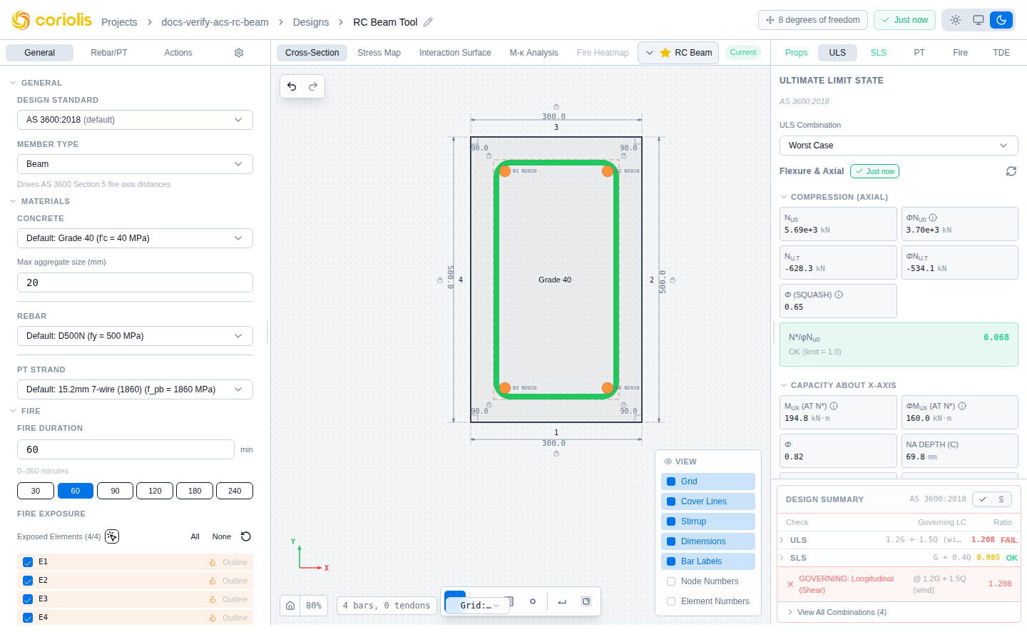
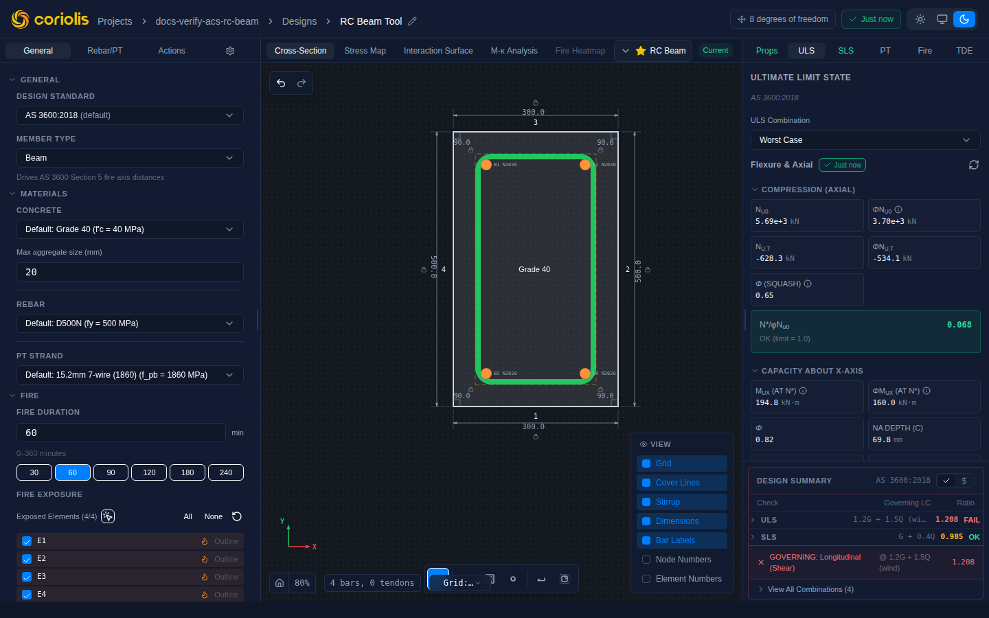
The flexure panel reports uniaxial bending capacity about the major () and minor () axes.
Capacity results
Key results:
| Output | Symbol | Units | Description |
|---|---|---|---|
| Pure-bending capacity (nominal) | kN·m | Moment capacity at zero axial load | |
| Pure-bending capacity (design) | kN·m | Design capacity at , after reduction | |
| Capacity at (nominal) | kN·m | Moment at which the section reaches ultimate strain at the applied axial | |
| Capacity at (design) | kN·m | Reduced capacity after applying at the applied axial | |
| Utilisation | — | Must be | |
| Neutral axis depth | mm | Depth of compression zone from the compression face | |
| Ductility parameter | or | — | Code-dependent ductility measure |
| Ductility status | — | — | Pass/fail against code limit |
ACS reports both / (pure bending, ) and / (at the actual applied axial ) for each load combination. This lets you read the full design curve directly: the design point (, ) is checked against at that specific level rather than the single-axis value.
Ductility applicability
The ductility checks below apply to a member declared as Beam or Slab in the General tab. A member declared Column or Wall does not get a Ductility status verdict — the panel instead shows an informational note, because reduced ductility for a compression member is carried by the capacity-reduction factor (Table 2.2.2) and the M–N interaction check, not the beam ductility limit.
The declared member type — not the axial load level reached by any combination — is what selects the check. When a declared Beam/Slab’s worst-case combination reaches column-level axial compression (, AS 3600 Cl. 10.3.2), or a declared Column/Wall never reaches it, ACS surfaces the disagreement as an advisory mismatch warning rather than silently switching which check runs — see Design Summary § Member type classification advisory.
Ductility checks by code:
| Code | Parameter | Limit | Reference |
|---|---|---|---|
| AS 3600 | (without compression steel) | Cl. 8.1.5 | |
| ACI 318 | (steel strain) | Cl. 21.2.2 | |
| EN 1992 | (typical) | Cl. 5.5 |
Compression-controlled classification
When the flexural ductility check fails — or when the neutral axis depth indicates a compression-controlled failure mode — ACS classifies the section explicitly:
| Classification | Meaning |
|---|---|
| Tension-controlled | Ductility satisfies the code limit; the full applies |
| Compression-controlled | Neutral axis depth exceeds the code ductility limit; is reduced (ACI 318) or the section is disallowed (AS 3600 Cl. 8.1.5) |
The classification is reported alongside the ductility parameter and status in the flexure panel.
Over-reinforced gate (AS 3600 Cl. 8.1.5)
When a section would be over-reinforced (i.e., with no compression steel, or the beam fails the conditional-use check), ACS enforces AS 3600 Cl. 8.1.5: the standard disallows use of the section unless compression reinforcement is added to satisfy the ductility limit. In this case:
- The flexure check reports a ductility failure, not a utilisation ratio.
- The result is disabled — displaying a capacity for an unconditional-use section would misrepresent the standard’s intent.
- Add compression bars to lower below the Cl. 8.1.5 limit.
This gate is scoped to a member declared as Beam or Slab (see Ductility applicability above); a declared Column or Wall is governed by Section 10 and the M–N interaction check instead, and never triggers the Cl. 8.1.5 use restriction.
Minimum bending strength (prestressed sections, AS 3600 Cl. 8.1.6.1(1))
For prestressed sections, ACS additionally checks that the pure-bending capacity is at least the minimum strength per AS 3600 Cl. 8.1.6.1(1). This check ensures the section has adequate residual strength after prestress-induced cracking.
Minimum flexural reinforcement
The section-level minimum reinforcement check uses the canonical flexural effective depth — the same value used by the per-combination flexural capacity analysis (distance from the extreme compression fibre to the centroid of the tension reinforcement). This ensures the minimum-steel check and the capacity result are always consistent, even for sections with mixed or non-standard bar layouts.
Min Reo panel
The Min Reo panel in the ULS results reports the minimum reinforcement check as a standalone result, separate from the flexural capacity utilisation:
| Output | Description |
|---|---|
| Required | Minimum area required by the governing code clause |
| Provided | Total tension reinforcement area |
| Utilisation | — must be for the check to pass |
| Status | Pass when provided area meets or exceeds the minimum |
Reporting minimum reinforcement as a dedicated panel ensures the failure is correctly attributed: a section that satisfies the flexural capacity check but provides insufficient reinforcement shows Min Reo: FAIL rather than attributing the failure to the flexure check. The flexural capacity result and the minimum reinforcement result are independent.
N-M interaction
For members under combined axial force and bending, the interaction diagram shows the full capacity envelope.
Uniaxial interaction plots the - curve with key points:
- Squash load: Pure compression capacity ()
- Balanced point: Simultaneous concrete crushing and steel yielding
- Pure bending (): Moment capacity at zero axial load
- Pure tension: Tensile capacity (reinforcement only)
Your design point () is plotted on the diagram. If it falls inside the envelope, the section is adequate. The and at values shown in the flexure panel correspond to the y-intercept and the design-point projection on the interaction surface respectively.
The interaction diagram reads directly from the design curve at the applied , per AS 3600 Interpretation B — not from the uniaxial value. This approach is consistent with how engineers read real interaction charts.
Biaxial interaction generates a 3D -- surface and checks the design point using:
- Rigorous method: 3D surface interpolation
- Bresler reciprocal (AS 3600 Cl. 10.6.4):
- Bresler load contour (ACI 318):
The biaxial check refuses axial demands that lie outside the squash-to-decompression range of the interaction surface. Providing a beyond the squash point triggers a clear error — ACS does not extrapolate capacity outside the envelope.
The interaction diagram can also be viewed as a 3D surface in the canvas Interaction tab.
Shear (AS 3600 Amendment 2:2021)
ACS implements the AS 3600:2018 Amendment 2:2021 shear model — a modified truss model with variable strut angle. This reconciliation was completed in the 2026 release wave and supersedes the pre-amendment implementation.
Shear capacity
Where:
- = concrete contribution, per the general method (Cl. 8.2.4.2) or simplified method (Cl. 8.2.4.3)
- = steel contribution,
- = web-crushing limit (Cl. 8.2.6), limiting the strut force
Method selection (AS 3600 Cl. 8.2.4.1)
ACS selects the shear method automatically:
- Simplified method (Cl. 8.2.4.3): , . Applicable when all of the following hold:
- No significant axial tension or torsion
- Concrete strength MPa
- Longitudinal reinforcement yield strength MPa
- Aggregate size mm
- General method (Cl. 8.2.4.2): Variable and derived from the longitudinal strain (Cl. 8.2.4.2.3). Used when any simplified-method condition above is not met, or when the member is subject to axial tension () or significant torsion.
When a combination includes a net tensile (positive = compression), or when the section material exceeds the concrete or steel strength limits, ACS switches to the general method automatically. A note in the shear results panel identifies which method is active for each combination.
Stirrup orientation and effective shear leg area
The ratio used in the steel shear contribution counts only the legs that are physically effective for the shear direction being checked. ACS resolves each stirrup’s contribution on a per-direction basis rather than using a simple leg count:
| Stirrup kind | V*y (crossing a horizontal shear plane) | V*x (crossing a vertical shear plane) |
|---|---|---|
| Rectangular hoop / perimeter | 2 legs | 2 legs |
| Crossties | $2 | \cos\beta |
| Diamond | Extent-averaged crossing count, area-weighted by inclination | Same, transposed to the horizontal direction |
| Helical / circular | 2 legs (rotation-invariant) | 2 legs |
A perfectly horizontal crosstie () contributes zero effective area to for the check — a horizontal bar cannot cross a horizontal shear crack. The same bar contributes its full leg area to the check. A diagonal crosstie contributes a partial area equal to its inclination projection to each direction.
Effective web width
The effective web width accounts for voided webs per AS 3600 Cl. 8.2.1.4. For hollow-core or box sections, ACS performs a horizontal scan to find the minimum solid material width at each web level. The scan is restricted to the flexural chord band — the material within the effective shear depth — so that a solid wedge or taper whose narrowest point lies outside is not credited with a vanishing . Restricting the scan can only raise the minimum, so the band relaxes an otherwise over-conservative full-extent value; for a prismatic web the two coincide exactly.
For prestressed sections, duct diameters are additionally deducted per AS 3600 Cl. 8.2.1.5. The deduction is evaluated per level, coupled to the width scan rather than applied to its result:
Where is the solid width at level , is the sum of prestressing duct diameters crossing that level, and is a deduction factor dependent on duct type. ACS applies the conservative ungrouted value . The deduction applies at a level only when .
Coupling the deduction to the level at which it occurs is the strict clause reading. It agrees exactly with the simpler decoupled form — minimum width, less the largest single-plane duct deduction — whenever the web is prismatic over the duct’s depth, which covers every prismatic ducted section. The two diverge only for a non-prismatic ducted web, where the narrowest level and the level carrying the largest are not the same: there, the decoupled form would subtract a deduction that never coincides with the true minimum width.
The same is threaded to both shear and torsion checks for consistency.
Aggregate size factor (general method)
The general method’s formula incorporates an aggregate size factor per Cl. 8.2.4.2(3)/(4):
When mm the formula gives exactly; for smaller aggregates increases (enlarging the denominator → reducing conservatively). For high-strength or lightweight concrete, the fixed value similarly reduces . When no aggregate size is specified, ACS defaults to mm.
Reinforcement yield strength cap
AS 3600 Table 3.2.1 limits the characteristic yield strength of shear reinforcement to 500 MPa, regardless of the bar grade specified. ACS enforces this cap in all AS 3600 shear calculations.
Transverse reinforcement limits
The minimum transverse reinforcement per AS 3600 Cl. 8.2.1.7 is:
The factor (general method) keys off the actual ratio compared to this , not a proxy value. The transverse-reo trigger applies the Cl. 8.2.1.6(1) depth factor when member depth exceeds the transition threshold.
Mandatory transverse reinforcement at D ≥ 750 mm (Cl. 8.2.1.6(3)): For beams with an overall section depth mm, AS 3600 requires transverse reinforcement meeting Cl. 8.2.1.7 minimum regardless of the computed shear demand. ACS checks this geometric threshold at the section level and flags the mandatory requirement in the shear results, independently of whether the applied would otherwise require stirrups.
The clause is scoped to beams and one-way slabs: this is selected by the declared Member Type in the General tab, the same declared-type basis as Ductility applicability above — not by the axial load level. A declared Column or Wall never triggers the mandatory requirement, regardless of section depth.
ACS reports:
| Result | Description |
|---|---|
| required | Stirrup area per unit length to satisfy |
| Minimum per Cl. 8.2.1.7 | |
| D ≥ 750 mm mandatory | Cl. 8.2.1.6(3) requirement (section-level, geometric trigger) |
| Governing requirement | Max of the above |
| Pass/fail | Whether the specified stirrups meet the governing requirement |
Reversal of loads (AS 3600 Cl 8.2.4.5)
AS 3600 Cl 8.2.4.5 states that where loading cases produce load reversal — causing flexural cracking in a zone that is usually in compression — may not apply and shall be assessed or taken as zero. The model assumes an intact compression zone and available aggregate interlock across diagonal cracks; load reversal degrades both mechanisms.
ACS evaluates the Cl 8.2.4.5 condition across the complete set of shear-carrying ULS combinations:
- Per-combination face cracking — a sagging moment cracks the bottom fibre when ; a hogging moment cracks the top fibre when . Cracking moments are axial-aware ( rises under net compression), so a prestressed zone that never actually cracks under the reversing moment retains its .
- Cross-combination detection — a combination is load-reversal affected when it cracks one face AND at least one other shear-carrying combination in the set cracks the opposite face. This both-faces requirement is faithful to the clause’s “usually in compression” criterion: if both faces are cracked across the set, whichever is usually in compression must have been cracked by the reversal.
- Conservative lower bound — for affected combinations, ACS sets so the capacity becomes only. The term continues to reflect any stirrups provided.
The check applies per shear axis: M*x combinations govern the V*y check; M*y combinations govern the V*x check.
A “Cl 8.2.4.5 reversal” note in the shear results panel identifies each affected combination and explains why was set to zero.
Biaxial shear ( and )
ACS checks shear separately on each principal axis. Enter (horizontal shear, crossing vertical planes) and (vertical shear, crossing horizontal planes) independently in the Applied Loads panel. Both axes are checked against the capacity computed for that direction; the governing axis controls the design.
Per-axis stirrup demand: is computed independently for the and checks using the directional leg areas described in Stirrup orientation and effective shear leg area above. The overall governing requirement is the maximum of the two axis demands (and the minimum).
Arc-section and curved-outline netting: For sections with curved outlines (circular, oval, arch), the net effective width at any scan level subtracts the displaced-concrete area attributable to curved boundaries using the same polygon-of-chords algorithm as the section property solver. Consequently, is always derived from the actual material extent at each level — not from a bounding-box approximation — which is conservative for thin-walled curved sections.
Combined capacity threshold: When both and are non-zero, ACS checks the vector resultant against to confirm the total demand does not exceed total capacity even when the individual axis utilisation ratios both appear moderate.
on both axes: The Cl. 8.2.1.7 minimum applies on each axis independently. A beam with significant must satisfy the minimum in the horizontal direction, even if is small.
Layered MCFT shear model
ACS implements a layered Modified Compression Field Theory (MCFT) solver alongside the code-simplified shear models. MCFT was originally developed by Vecchio & Collins (1986) and was subsequently codified in CSA A23.3. The layered variant divides the section into a stack of horizontal layers and applies MCFT equilibrium and compatibility at each layer independently, accounting for the actual transverse reinforcement content and concrete properties at every level.
How it works
- Section discretisation — the cross-section is divided into thin horizontal layers (default: 50 layers, or a user-adjusted count). Each layer carries its local concrete area, any reinforcement crossing that layer, and the applied axial strain from the global N- state.
- Per-layer MCFT — within each layer, the MCFT compatibility equations (principal strain directions) and equilibrium equations (stress resultants) are solved iteratively. The principal compressive stress direction is free to vary between layers, so it is not forced to match the global truss-angle assumption.
- Transverse reinforcement content — the effective transverse reinforcement ratio is resolved per layer from the stirrup cross-section area present at that level. For uniform stirrup layouts the per-layer equals the global ; for non-uniform or bundled transverse steel it differs layer by layer.
- Aggregate — the per-layer shear stress contributions are integrated across the section depth to produce the total concrete shear capacity and the required transverse steel demand.
Compression base curve
The MCFT compression stress-strain law used for each layer’s principal compressive direction is controlled by the base curve setting. Two curves are available:
| Curve | Formula | Notes |
|---|---|---|
| Popovics (default) | Thorenfeldt–Collins–Mitchell per Bentz thesis §5: empirical MPa; peak strain ; shape factor ; post-peak decay | Recommended by Bentz (Response-2000). No finite crush strain — the march terminates when turns over. |
| Parabolic | Vecchio & Collins 1986: , , fixed | Exhausts at (crush exit). |
Compression softening (Vecchio & Collins 1986 ) is orthogonal to the base curve choice and applied to both.
Self-consistency criterion
After the capacity march finds a candidate peak, the solver verifies that the accepted inner state is a genuine fixed point of the MCFT equations, not the collapsed zero-support absorbing state (a spurious self-reproducing solution that can produce V ≈ 0).
The criterion is the maximum shear-stress profile mismatch between the last shape-function iteration (LSM) and the MCFT back-calculation:
A state is accepted only when . The collapsed attractor produces mismatches of 2.4–11.4 MPa — well above the threshold — so it is reliably excluded. A consistent branch solution sits at .
The march diagnostics record PeakTauMismatchMPa for the accepted peak and expose it in the analysis detail panel. Values above 0.08 MPa indicate a non-convergent state; the solver reports no capacity for that load step rather than returning a result that fails the criterion.
Correctness improvements (2026)
Five solver issues were corrected in the 2026 release wave:
- Cracking-transition solver rework — the iterative solver previously used a fixed cracking-moment threshold that did not account for axial force when determining which layers had transitioned from uncracked to cracked. The reworked solver evaluates the cracking condition per-layer using the axial-aware formula, eliminating false-cracked and missed-cracked layers under combined N+M.
- Per-layer resolution — the transverse reinforcement ratio was previously computed once at the centroidal level and applied uniformly to all layers. The solver now resolves individually for each layer from the stirrup geometry intersected at that height. Results for sections with non-uniform transverse reinforcement (tapered stirrups, variable-spacing zones, bundled links) will differ from pre-fix results.
- Collapsed-attractor fixed-point guard (#3521) — a zero-support absorbing state that self-reproduced through the corroboration certificate (producing spurious near-zero capacities on high-utilisation sections near mechanism) was identified and closed by the self-consistency criterion above. Results for sections that previously returned an abnormally low or zero MCFT capacity may be corrected upward.
- ρ=0 transverse reinforcement bracket degeneracy (#3553) — when no transverse reinforcement was present (), the root-finding bracket degenerated to a zero-width interval and convergence failed. The bracket lower bound is now seeded from the concrete shear contribution alone, giving the solver a non-degenerate starting interval for unreinforced sections.
- Branch-jump guard (#3559) — the capacity march’s peak-detection step previously accepted candidates located on a different solution branch than the one traced during the ascending sweep, producing a discontinuous jump in reported capacity at branch crossings. A continuity check now rejects off-branch candidates; the march progresses on the original branch and accepts only peaks reached by monotone progression along that branch.
:::note Results computed before 2026-07-17 may differ from results computed on or after that date. Two changes land simultaneously: the base curve switch from Parabolic to Popovics (which shifts for all sections) and the fixed-point guard (which corrects the collapsed-attractor failure class). For sections that were not affected by the attractor bug, the Popovics curve itself produces a continuous curve with no finite crush exit, typically yielding slightly higher than the parabolic curve for normal-strength concrete. If you have previously calculated results that are used in a design submission, re-run the analysis and compare.
Additionally, results computed before 2026-07-18 may differ for sections with zero transverse reinforcement () — where the bracket degeneracy fix lands — and for sections where the capacity march previously selected a peak on an off-branch root. Re-run shear analyses for these cases and compare. :::
:::note For sections with uniform transverse reinforcement — constant-diameter, constant-spacing stirrups running the full section depth — the per-layer and the global are identical and numerical results are unchanged by that specific fix. :::
When to use the layered model
The layered MCFT is most beneficial when:
- Transverse reinforcement varies over the section depth (e.g. additional horizontal bars in the web, tapered-leg stirrups, or multiple stirrup sizes).
- The section has a non-rectangular profile (T-beams, I-sections) where the effective width changes significantly with height.
- A research-grade or peer-review deliverable requires a more theoretically rigorous shear model than the code-simplified approach.
For routine AS 3600 design, the Amendment 2 general method described above is the governing code check. The layered MCFT result is reported as a secondary output alongside the code check and does not replace it.
Shear (EN 1992-1-1:2004)
For sections designed to EN 1992-1-1, ACS implements the variable-strut-angle model from Cl. 6.2.2 and Cl. 6.2.3.
Concrete contribution (Cl. 6.2.2)
For members without shear reinforcement:
Where:
- (size effect factor, in mm)
- (longitudinal tension reinforcement ratio)
- (average axial stress; positive = compression)
- , (recommended values from the National Annex)
has a minimum: where .
Steel contribution (Cl. 6.2.3)
For members with shear reinforcement (variable-strut-angle truss):
Where:
- = strut angle, constrained to (i.e. )
- = axial-force coefficient: for non-prestressed; rises to for ; peaks at for ; reduces to for
- = strength reduction factor for concrete cracked in shear ()
- (lever arm; ACS uses the exact computed value)
Strut-angle crossover: The optimal (minimising ) is found from the point at which and are both exactly equal to . ACS solves this crossover analytically so the strut angle is never under- or over-optimised.
Axial tension (): The term with reduces ; drops below 1.0 proportionally, reducing .
Torsion
For members with applied torsion , the combined shear-torsion check follows AS 3600 Cl. 8.2.5.3. The transverse-steel demand from shear and torsion is summed directly, and the section must satisfy the combined requirement simultaneously.
The same effective web width and strut angle used for shear are applied to the torsion checks, keeping the two checks in lockstep.
Longitudinal chord check (AS 3600 Cl. 8.2.7.1(2))
For members resisting shear without torsion, AS 3600 Cl. 8.2.7.1(2) requires that longitudinal bars be checked against the additional tensile (or compressive) chord force induced by the shear truss mechanism:
Where:
- = vertical component of prestress force (zero for non-prestressed sections)
- = strut angle from the governing shear check
ACS reports the chord force ratio for each face — the governing ratio (tension or compression side) must be ≤ 1.0 for the check to pass. This check sits alongside the flexure utilisation, so total longitudinal bar demand is the sum of bending plus chord tension.
ULS Stress Map
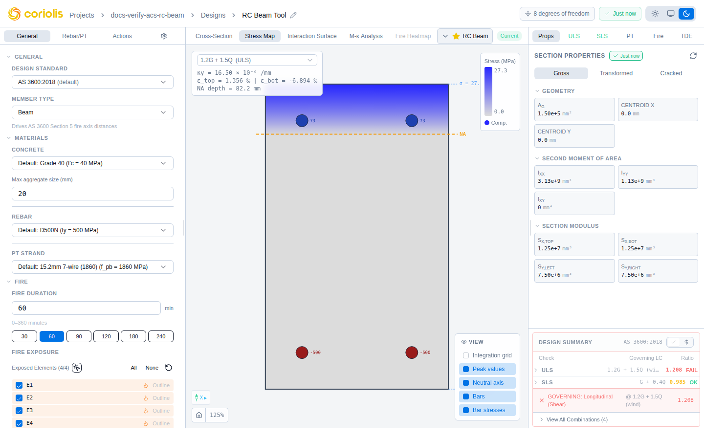
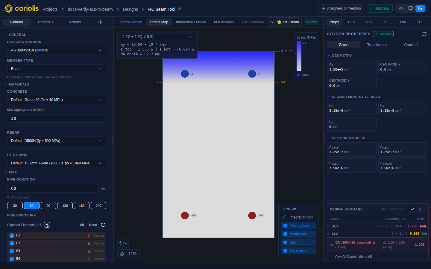
The Stress Map tab in the canvas visualises the computed stress field across the section at the selected ULS design point (). The fibre solver locates the neutral-axis position that equilibrates the applied actions, then evaluates the stress at each integration point; a continuous colour gradient maps this over the section outline. The biaxial stress-distribution grid is clipped to the section polygon — fibres outside the concrete boundary are excluded — so the visualisation accurately represents the stress state within the material.
Convergence gate: The Stress Map renders only when the fibre solver successfully converges to the target design point. When convergence fails — for example, a heavily pre-compressed section where the equilibrium curvature falls below zero for a given moment demand — ACS shows an error state rather than displaying a non-equilibrium stress overlay. This prevents incorrect data from reaching the user when a valid result cannot be computed.
:::tip[New: the Stress Map can now be zoomed] The Stress Map previously rendered at a fixed fit-to-window scale with no way to get closer. It is now a full viewport: scroll to zoom, middle-drag or Ctrl (⌘) + left-drag to pan, and the house icon in the bottom-left corner to reframe the whole section.
Use it to inspect stress concentrations near individual bars or at section corners. The neutral-axis line, bar markers and labels are vectors and stay sharp at any zoom; the stress field itself is redrawn at full resolution a moment after you stop zooming. :::
The full control set, which is shared with every other canvas in the platform, is in Canvas navigation.
Serviceability limit state (SLS)
SLS checks use the first active SLS load combination.
Stress check
Verifies that concrete and steel stresses under service loads remain within allowable limits:
| Check | Limit (AS 3600) | Limit (ACI 318) | Limit (EN 1992) |
|---|---|---|---|
| Concrete compression | |||
| Steel tension |
The AS 3600 steel stress limit is capped at MPa due to the 500 MPa yield-strength cap, even when a higher-grade bar is specified.
An SLS Stress Field tab in the canvas visualises the computed stress distribution at service load, using the same biaxial fibre integration approach as the ULS Stress Map. Its grid is likewise clipped to the section polygon so that only fibres within the concrete boundary contribute to the colour field.
Crack width
Computes the characteristic crack width and compares it against the allowable width for the exposure class:
Where:
- = maximum crack spacing
- = mean steel strain
- = mean concrete strain between cracks
AS 3600 strain term (Cl. 8.6.2.3(2)): Uses a fixed 0.6 tension-stiffening coefficient, mean axial tensile strength , effective modular ratio , and — on long-term SLS combinations — the final design shrinkage strain . Long-term crack widths are therefore substantially larger than short-term ones. The steel crack-inducing stress is capped at per Cl. 8.6.1 — this prevents the crack-width result from being under-stated when the bar stress approaches yield.
EN 1992-1-1 strain term: -parametrised (0.4 long-term / 0.6 short-term, no shrinkage term). EN 1992 crack widths do not grow significantly with duration beyond the adjustment.
Typical limits: 0.3 mm for sheltered environments, 0.2 mm for exposed, 0.1 mm for water-retaining.
EN 1992-1-1 crack control for prestressed members (Cl. 7.3.1, Table 7.1N)
For sections with prestressing tendons, EN 1992-1-1 applies tighter crack control requirements than for ordinary reinforced concrete. ACS implements the full Cl. 7.3.1(6) framework:
Exposure-class limits (Table 7.1N):
| Exposure class | Prestressed members — recommended |
|---|---|
| X0, XC1 | 0.2 mm (under quasi-permanent loads) |
| XC2, XC3, XC4 | 0.2 mm (under quasi-permanent loads) |
| XD1, XD2, XS1, XS2, XS3 | Decompression check (no cracking under quasi-permanent loads) |
For the XD/XS exposure classes, decompression is the limit state — every fibre in the cross-section must remain in compression (or at least at zero stress) under the quasi-permanent combination. ACS performs the decompression check for bonded tendons within 100 mm of the exposed surface, as specified in Cl. 7.3.1(6).
Mechanism A — stress increment (Cl. 7.3.4):
For bonded post-tensioned sections that are designed to remain uncracked (decompression governs), ACS verifies the tendon stress increment between the decompression load level and the characteristic load combination:
Where is the additional strain in the prestressing steel above the decompression state. EN 1992-1-1 limits (nationally determined parameter; default 200 MPa for post-tensioned, 150 MPa for pre-tensioned) to guard against fatigue at the decompression cycle under traffic or variable loading.
Scope note: Crack width calculation for cracked prestressed sections under EN 1992-1-1 (i.e. when the cross-section is in tension under the quasi-permanent combination and Table 7.1N’s limit applies) uses the same and expressions as for reinforced concrete with the contributing bonded tendon area added to . Support for combined bonded-tendon-plus-bar crack width in the cracked regime is pending — see Prestressing for current scope.
Deflection parameters
Computes the effective moment of inertia for deflection calculation:
Where:
- = gross moment of inertia
- = cracked moment of inertia
- = cracking moment
- = service moment
Long-term factors account for creep and shrinkage effects.
Prestressing
See the dedicated Prestressing page for the full workflow. A summary of the key checks:
For sections with tendons, the PT tab provides:
Prestress losses
All loss components are computed individually:
| Loss type | Category | Reference |
|---|---|---|
| Elastic shortening | Immediate | AS 3600 Cl. 3.4.3.3 |
| Friction | Immediate | AS 3600 Cl. 3.4.3.1 |
| Anchorage draw-in | Immediate | AS 3600 Cl. 3.4.3.2 |
| Creep | Long-term | AS 3600 Cl. 3.1.8 |
| Shrinkage | Long-term | AS 3600 Cl. 3.1.7 |
| Relaxation | Long-term | AS 3600 Cl. 3.3.4.3 |
The effective prestress after all losses is used for subsequent capacity and stress checks.
Transfer and service stresses
Concrete stresses are checked at two stages:
- Transfer: immediately after prestressing (using , the concrete strength at transfer)
- Service: long-term under sustained loads (using )
Extreme-fibre distances and section moduli used in the fibre stress calculation are measured from the transformed centroid — the centroid of the composite transformed section including the modular-ratio contributions of all steel and tendon areas. This correctly accounts for the shift in neutral axis from gross to transformed geometry for PT sections.
PT ultimate capacity
The moment capacity of the prestressed section accounts for tendon stress increase beyond the effective prestress. PT ultimate capacity uses the effective (post-loss) prestress as the starting point — not the jacking stress — ensuring the analysis matches the actual in-situ tendon state:
Where is the additional strain at the tendon level at ultimate, capped at .
Fire design
See the dedicated Fire design page for detailed documentation.
Moment-curvature analysis
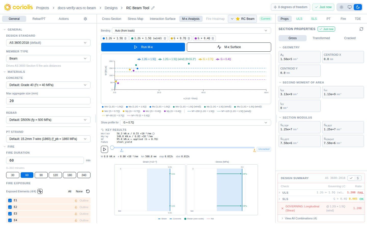
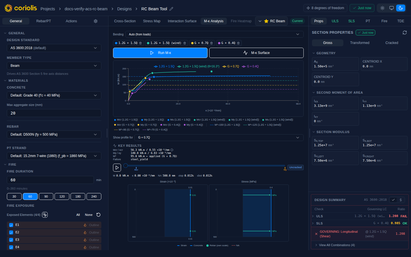
The Moment-curvature tab traces the full nonlinear response of the section:
- Uncracked elastic phase
- Cracking (concrete tensile strength exceeded)
- Post-cracking (tension stiffening)
- Steel yielding
- Ultimate (concrete crushing or steel rupture)
The M- curve shows ductility capacity and energy absorption. You can run curves at multiple axial load levels and view the results overlaid on the same plot.
The M- interaction surface (triggered by button) generates a 3D surface by sweeping the bending angle from 0° to 360° at multiple axial load levels. This provides a rigorous biaxial interaction check based on the full nonlinear material response.
Design summary
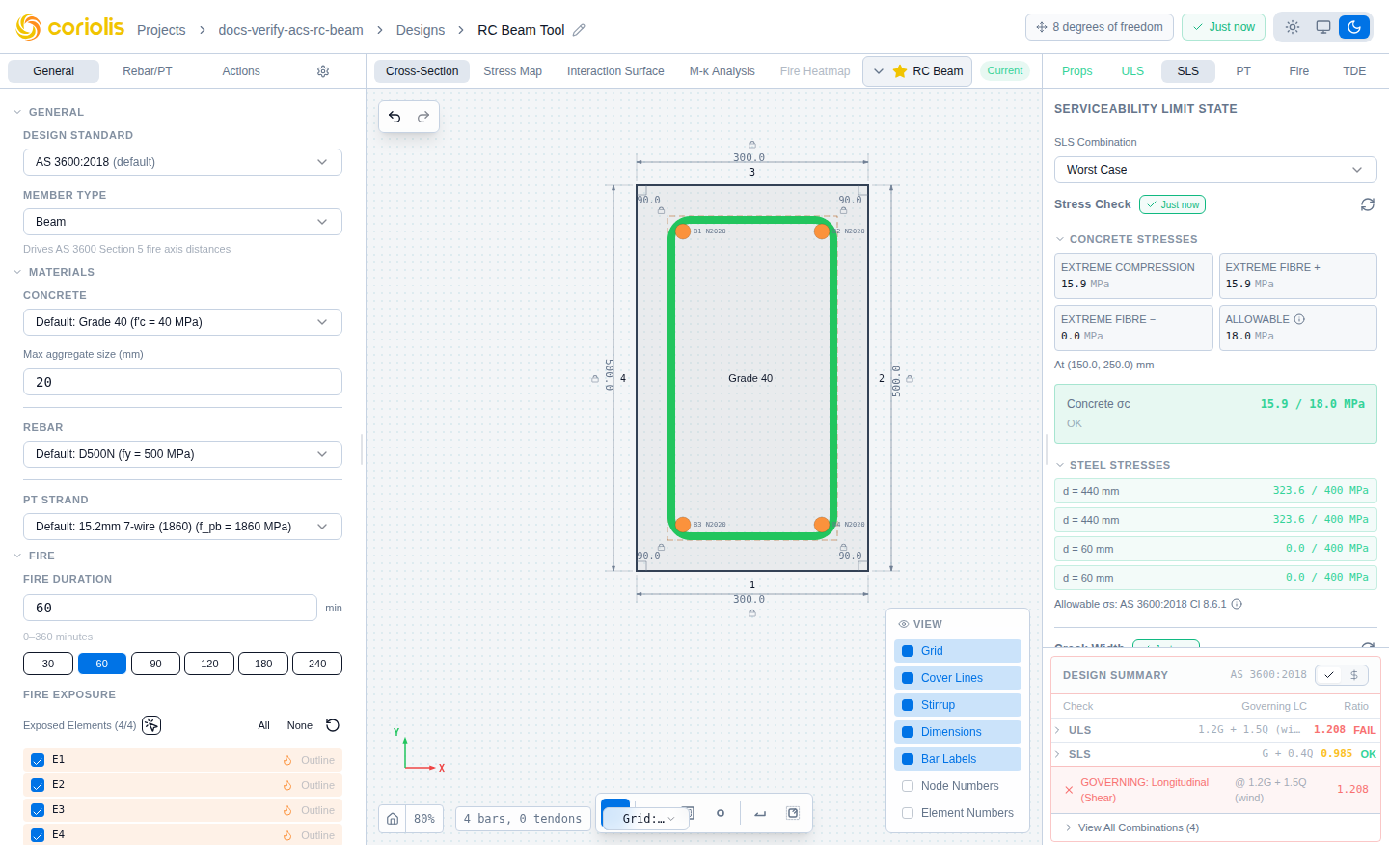
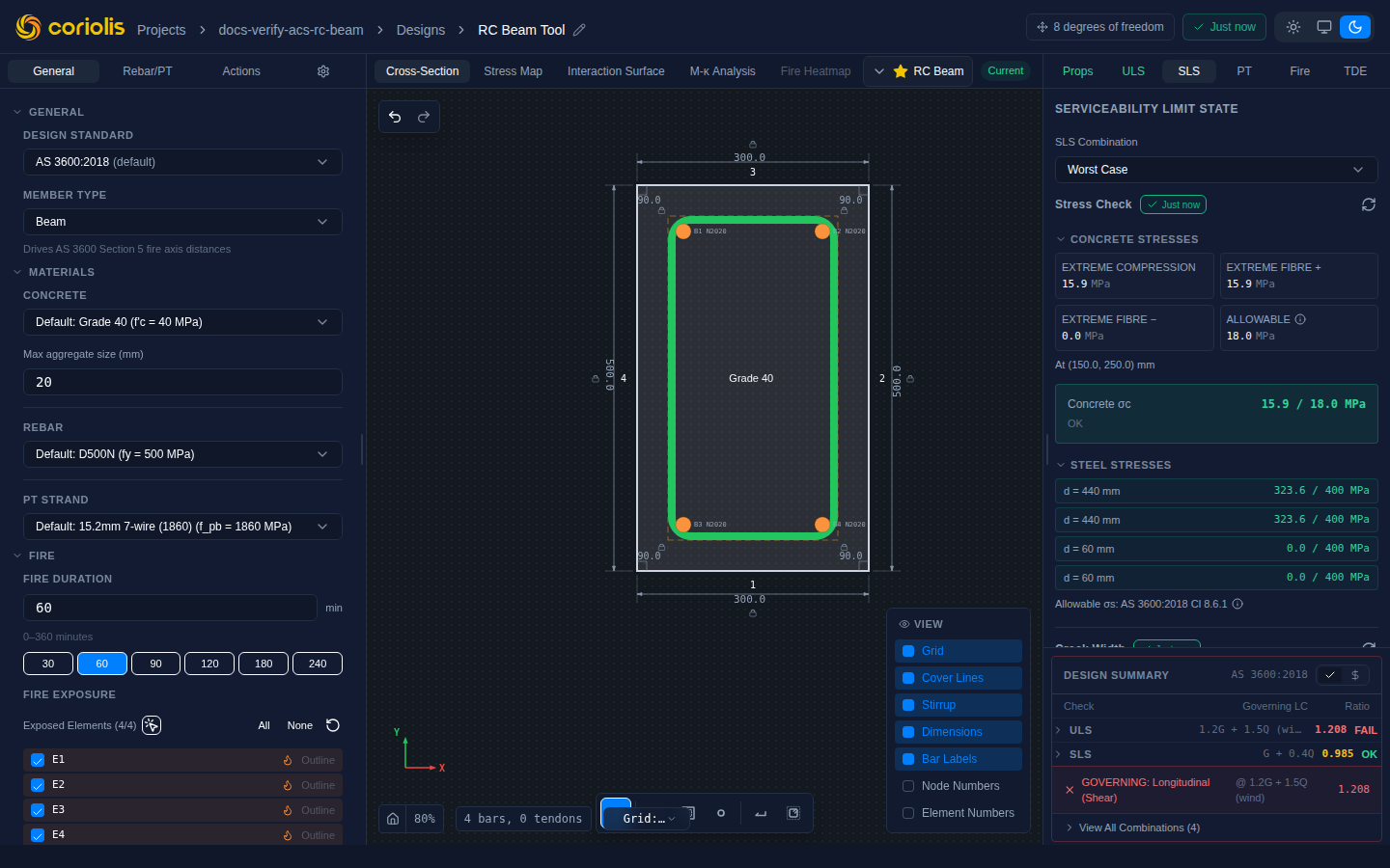
The Summary tab collects all ULS, SLS, and fire check results into a collapsible accordion panel. Each accordion group covers one check category and shows a Category Rollup badge — the worst utilisation ratio across all load combinations in that group — so you can scan the full design status without expanding every section. Groups are collapsed by default.
The View All Combinations section at the bottom expands to a matrix table of every load combination against every check type, making it easy to spot combinations that govern multiple checks simultaneously.
Material quantities (concrete volume, reinforcement mass per unit length) appear below the check results. If the section geometry contains a NaN or infinity coordinate, the quantities panel shows an explanatory error rather than propagating meaningless values — see Design Summary § Non-finite coordinate guard.
The ULS group may also carry a member type classification advisory — a note disclosing when the declared Member Type disagrees with the load level reached across the ULS envelope (see Ductility applicability above and Design Summary § Member type classification advisory).
See the Design Summary page for full documentation of the panel layout, accordion groups, View All Combinations matrix, and material quantities.
Time-dependent effects
See the dedicated Time-dependent effects page for creep and shrinkage analysis using the age-adjusted effective modulus method (AEMM).
Related pages
- Design Summary — panel layout, accordion groups, and View All Combinations matrix
- Fire design — fire rating analysis
- Prestressing — tendon definition, losses, transfer/service stresses
- Time-dependent effects — creep and shrinkage analysis
- Moment-curvature theory — mathematical background
- M-N interaction theory — interaction diagram theory
- Creep and shrinkage theory — AEMM background
- Design standards — AS 3600 vs ACI 318 vs EN 1992 comparison
- RC beam worked example — step-by-step design