Worked example: composite section

Build a steel-on-concrete composite section in the Section Analyzer — a 200 × 50 mm concrete slab with a 100 × 150 mm steel beam stacked on top — and walk through both the geometric and stiffness-weighted (transformed) property output.

Problem statement

We want to analyse a simple composite cross-section: a 200 × 50 mm concrete slab with a 100 × 150 mm steel beam stacked on top of it. This is the textbook composite-beam configuration — the concrete bears in compression while the steel carries tension (and bending stiffness). The two regions are touching at the slab–beam interface but do not overlap.

We want:

The geometric section properties — treating both regions as a single 2D shape, with no material weighting
The stiffness-weighted (transformed) properties — referenced to the concrete

This example walks through the adjacent regions composite layout — two outlines of different materials that share a boundary but no interior area. The embedded inclusion layout (inclusion strictly inside an outline — rebar inside concrete) is planned but not yet shipped: the region validator currently rejects any outline+inclusion overlap, including strict containment, with overlapping_regions. Tracking issue: #1748. The intended behaviour (and what the modular-ratio bookkeeping will look like when it lands) is sketched at the end of this page for reference.

Given data

Region	Role	Geometry (mm)	Material	$E$ (MPa)
1	Outline	Concrete slab — 200 × 50 with bottom-left at $(0, 0)$	AS 3600 Grade 32	33,000
2	Outline	Steel beam — 100 × 150 with bottom-left at $(50, 50)$	Steel (Grade 350)	200,000

Modular ratio of steel to concrete: $n_s = E_s / E_c = 200{,}000 / 33{,}000 \approx 6.061$ .

Step 1 — Draw the concrete slab

Open the Section Analyzer for a new design option. Press P to enter Draw Polygon mode and draw the 200 × 50 rectangle at the origin. Use SHIFT-and-distance-lock for exact dimensions.

In the Elements list set the role of the new element to Outline and assign AS 3600 Grade 32 as the material.

Step 2 — Draw the steel beam

Press P again and draw the 100 × 150 rectangle starting at $(50, 50)$ . Set its role to Outline and assign Steel (Grade 350) as the material.

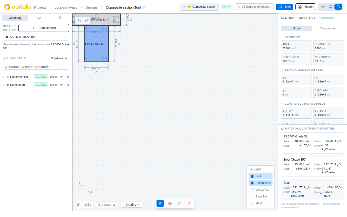
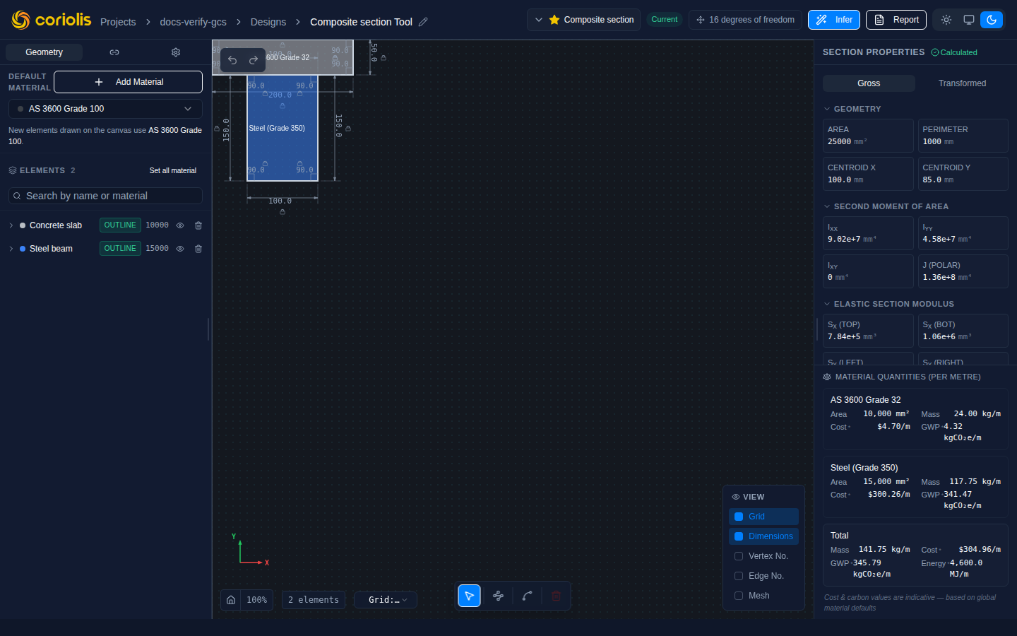
The two rectangles meet along the segment from $(50, 50)$ to $(150, 50)$ . The validator allows shared boundaries; what it rejects is interior overlap. This boundary-touching is the adjacent condition the composite model is built around.

The composite section after drawing both regions — the concrete slab on the bottom and the steel beam stacked on top, sharing the interface line at y = 50.

Step 3 — Read the analysis output

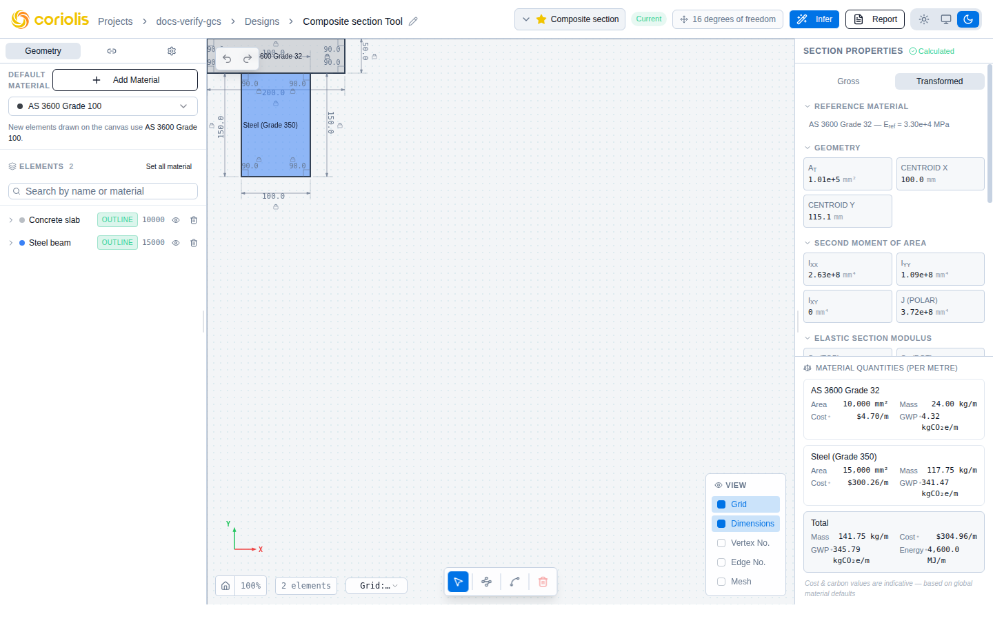
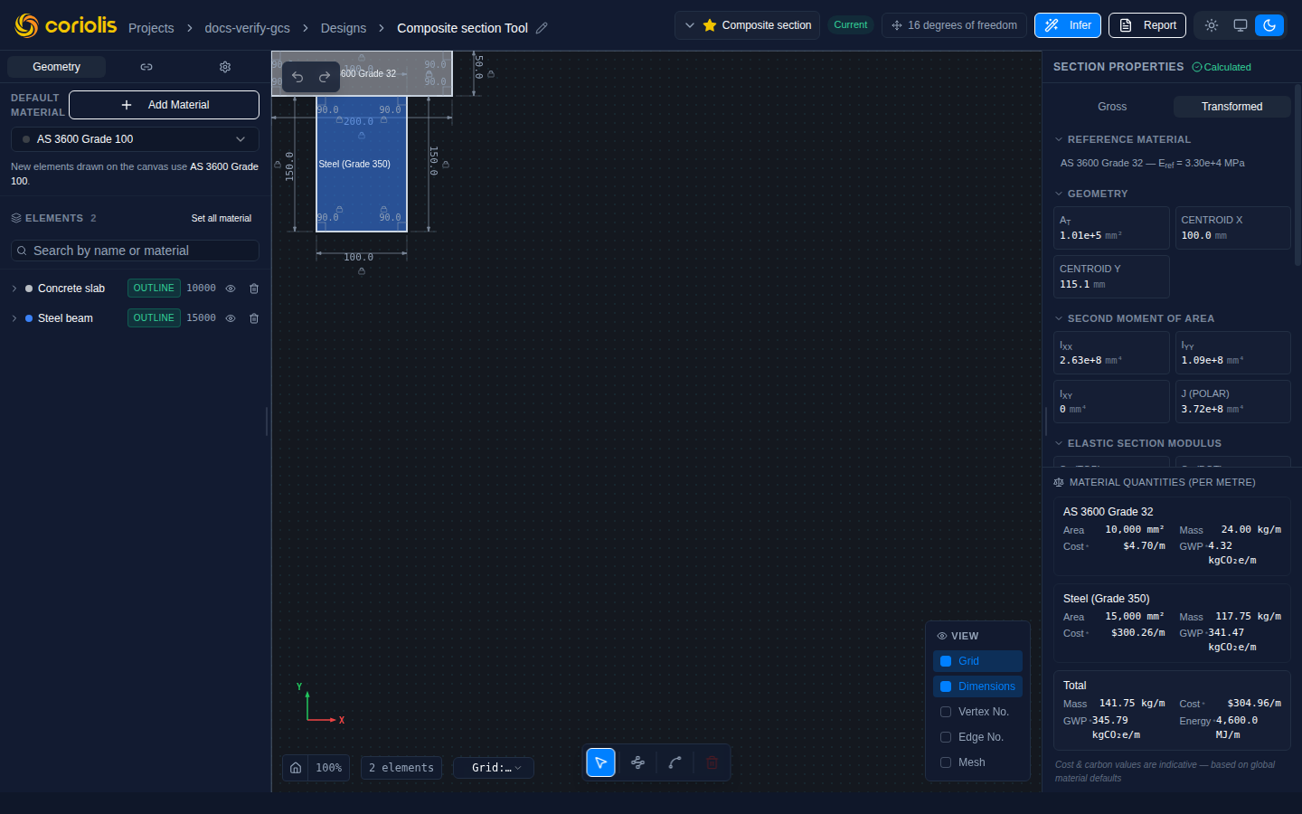
As soon as the geometry validates server-side the badge in the sidebar header flips from Preview to Calculated. The properties panel now shows two groups: the geometric properties at the top (which sum both rectangles as one shape with no material weighting), and the transformed properties below (which scale the steel’s contribution by the modular ratio).

The right-sidebar Section Properties panel showing the geometric properties at the top and the stiffness-weighted (transformed) properties below — each group has its own area, centroid, and second moments.

Geometric properties (what the canvas shows as the section)

These properties treat both regions as a single shape — material assignments do not enter the calculation here.

Property	Symbol	Value
Total area	$A$	25000 mm²
Perimeter	$P$	1000 mm
Centroid $x$	$\bar{x}$	100 mm
Centroid $y$	$\bar{y}$	85 mm
Second moment about $x$	$I_{xx}$	9.02e7 mm⁴
Second moment about $y$	$I_{yy}$	4.58e7 mm⁴

Hand check — area and centroid

$A = A_\mathrm{slab} + A_\mathrm{beam} = (200)(50) + (100)(150) = 10{,}000 + 15{,}000 = 25{,}000 \text{ mm}^2$

The two regions are both symmetric about $x = 100$ , so the geometric centroid sits on that axis: $\bar{x} = 100$ mm.

For the $y$ centroid, take area-weighted moments about the bottom edge:

$\bar{y} = \frac{A_\mathrm{slab}\,\bar{y}_\mathrm{slab} + A_\mathrm{beam}\,\bar{y}_\mathrm{beam}}{A_\mathrm{slab} + A_\mathrm{beam}} = \frac{(10{,}000)(25) + (15{,}000)(125)}{25{,}000} = \frac{250{,}000 + 1{,}875{,}000}{25{,}000} = 85 \text{ mm}$

The reported value matches.

Hand check — second moment $I_{xx}$

Apply the parallel-axis theorem for each region about the composite centroid ( $\bar{y} = 85$ mm):

$I_{xx,\mathrm{slab}} = \frac{b h^3}{12} + A\,d^2 = \frac{(200)(50)^3}{12} + (10{,}000)(25 - 85)^2 = 2.083 \times 10^6 + 3.60 \times 10^7 = 3.808 \times 10^7$

$I_{xx,\mathrm{beam}} = \frac{(100)(150)^3}{12} + (15{,}000)(125 - 85)^2 = 2.813 \times 10^7 + 2.40 \times 10^7 = 5.213 \times 10^7$

$I_{xx} = 3.808 \times 10^7 + 5.213 \times 10^7 \approx 9.02 \times 10^7 \text{ mm}^4$

Matches the reported value.

Transformed (stiffness-weighted) properties

The first outline (the concrete slab) sets the reference material. The steel beam’s contributions are scaled by the modular ratio $n_s = 6.25$ .

Property	Path	Notes
Reference material	`transformed.referenceMaterial`	AS 3600 Grade 32, $E = 33{,}000$ MPa
Transformed area	100909 mm²	$A_c + n_s\,A_s = 10{,}000 + 6.061(15{,}000)$
Transformed centroid $y$	115.09 mm	Steel pulls the elastic neutral axis upward toward the steel beam
Transformed second moment $I_{xx}$	2.626e8 mm⁴	Much larger than $I_{xx}$ above because the heavily weighted steel is far from the transformed centroid

Hand check — transformed centroid

Take E-weighted moments about the bottom edge:

$\bar{y}_t = \frac{A_c \bar{y}_c + n_s\,A_s\,\bar{y}_s}{A_c + n_s\,A_s} = \frac{(10{,}000)(25) + (6.061)(15{,}000)(125)}{100{,}909} = \frac{250{,}000 + 11{,}363{,}636}{100{,}909} \approx 115.09 \text{ mm}$

Notice how much the centroid shifts compared with the geometric one ( $\bar{y} = 85$ mm). The steel’s stiffness pulls the elastic neutral axis toward it by about 30 mm — and this is exactly why composite design uses transformed properties: stress and strain at any fibre are governed by the transformed centroid and transformed $I$ , not by the geometric values.

Plastic modulus is null

Both plasticModulus and shapeFactor are null in the response, with plasticModulusReason explaining why. Composite plastic capacity depends on per-material yield, not on modular ratio — the Section Analyzer refuses to substitute a meaningless value. See Materials — Plastic modulus is null for composite sections. For plastic capacity of this composite as a real structural element, use a material-specific designer.

What this example demonstrates

The composite model is built around the adjacent-regions layout. Two outlines sharing a boundary but no interior area. The embedded-inclusion layout (next section) is the planned extension under #1748 — today the validator rejects any outline+inclusion overlap (including strict containment) with overlapping_regions.
Geometric and transformed properties answer different questions. Geometric properties describe the shape; transformed properties capture how the composite responds to bending under linear-elastic behaviour.
The reference material is explicit in the response. You never have to guess what stiffness the transformed properties are expressed in.
Plastic capacity is not in scope for composite sections in this tool — see the scope statement for the reasoning.

Embedded inclusions — rebar inside concrete (planned — tracked at #1748)

The Section Analyzer does not support embedded inclusions today — the region validator rejects any outline+inclusion overlap (including strict containment) with overlapping_regions. The sketch below describes the intended behaviour once #1748 lands, so consumers of the docs know what is coming. For embedded-reinforcement workflows today, use the Advanced Concrete Section, which solves the same and richer problem with proper strain compatibility.

When #1748 lands, the workflow will look like this — consider a single concrete outline with a steel inclusion strictly contained inside it:

Draw a 200 × 100 concrete Outline at the origin.
Draw a 20 × 20 steel Inclusion with its centre at the outline’s centre — for example bottom-left at $(90, 40)$ . Set the role to Inclusion and assign Steel (Grade 350).
The section properties panel will update automatically as soon as the geometry validates.

The geometric properties will be unchanged from the bare outline — the inclusion will displace the host material at its footprint, so $A = 200 \times 100 = 20{,}000\ \text{mm}^2$ . The transformed properties will pick up the extra stiffness of the embedded steel:

$A_t = A_\mathrm{outline} + (n_s - 1)\,A_\mathrm{inclusion} = 20{,}000 + (6.061 - 1)(400) \approx 22{,}024\ \text{mm}^2$

Equivalently: the host material will own the displaced footprint at modular ratio 1, the inclusion will replace it at modular ratio $n_s$ , and the difference is $(n_s - 1)\,A_\mathrm{inclusion}$ . The same arithmetic will carry through the second-moment and centroidal integrals.

This will be the right tool for the linear-elastic stiffness-weighted properties of a reinforced section once it ships. For full RC design (concrete cracking, rebar yielding, $M$ – $N$ interaction, biaxial bending), the Advanced Concrete Section is still the right destination — the modular-ratio method here cannot capture post-elastic behaviour. Both tools will complement each other rather than substitute.

Where to go next

Section properties reference — the full output catalogue with formulas
ACS — for reinforced concrete design (post-elastic, code-capacity)
Limitations — what the analyser deliberately does not do